Diffusion Language Models -- Part Four (Post-training with Reinforcement Learning)

October 4, 2025

⊕
Source: PNGs in GIF generated with ChatGPT.

Recently, the post-training of large language models (LLMs) with reinforcement learning (RL) has been an important source for the significant progress we are seeing in LLM capabilities (for reasoning, agents/tool-use, planning etc).

⊕The post-training of an LLM comes after pretraining (which is when LLMs are trained on next-token prediction over web-scale text). It “polishes” the LLM into the useful models we are used to interacting with. This blog post by two Meta Super Intelligence (MSL) researchers gives a good overview of the post-training phase. Much of what is in their blog post would also apply to post-training for diffusion language models (DLMs).

This became especially apparent earlier this year when DeepSeek surprised (and moved markets) with the release of their R1 model (Guo et al, 2025), an auto-regressive LLM (AR-LLM). Their model was post-trained with an efficient RL algorithm (GRPO, see below) in a way that unlocked “thinking” for improved performance on reasoning tasks.The term ‘reasoning’ with respect to LLMs, also referred to as Large Reasoning Models or LRMs, is still being settled upon. However, there are notable differences between the “thinking” traces produced by LRMs and what we might generally accept as reasoning by humans. A good overview of this can be found in (Kambhampati et al, 2025) and this list. Prior to this, however, RL post-training was already crucial for aligning AR-LLM generations towards users’ preferred forms/styles of text and conversation, as well as for meeting safety and security requirements.

In this post, I examine similar RL methods for diffusion language models (DLMs); which will be key for pushing DLMs to parity (or more) with existing AR-LLMs in terms of capabilities. In line with the previous posts of this series, I will focus on Masked-DLMs (which are the keenest focus of current research); on the RL side, my focus will be on online policy-gradient algorithms,Policy-gradient algorithms are named for how: (i) the policy (the mechanism for generating trajectories i.e. sequences of tokens when used in the context of LLM RL post-training) is in the form of a parameterized model, and (ii) the policy’s parameters are learned by following the gradient of some function with respect to those parameters. (The definitions of the terms in red can be found below.) They can be categorised as being online or offline, where the “on”/”off” relates to whether the policy is learning from trajectories coming from itself (“on”) or not (“off”; e.g. from another model’s distribution).

Sidenote: offline methods, such as DPO (Rafailov et al, 2023), were instrumental for aligning LLM to human preferences (e.g. used in the training for Llama 3 (Llama Team, AI @ Meta, 2024) models). For the interested, similar methods have been proposed for diffusion models: e.g. VRPO used to post-train the original LLaDA Masked-DLM (Nie et al, 2025) to give LLaDA 1.5 (Zhu et al), as well as ones for continuous diffusion such as Diffusion-DPO (Wallace et al, 2023) and DSPO (Zhu et al, 2025). namely: Group Relative Policy Optimization (GRPO) (Shao et al, 2024), (DeepSeek AI, 2025) and Proximal Policy Optimization (PPO) (Schulman et al, 2017), which (i) are being used in post-training AR-LLM today; and (ii) have been found to reach better performance compared to offline algorithms (Ivison et al, 2024).

The outline of this post is as follows: I will start by setting the scene with 1. an accessible introduction to RL post-training using policy-gradient algorithms, followed by outlining 2. the main challenge for DLM post-training with such methods. I will then highlight 3. some proposed approaches for RL post-training of DLMs. If you are familiar with RL post-training for LLMs, you could just skip directly to section 2. Otherwise, to fully benefit from this post, going through my earlier posts Part 1, Part 2 and Part 3 for some background to DLMs first would probably be useful.

🖼️ 1. Paint a picture of RL post-training of LLMs in 5 minutes?

Before discussing policy-gradient RL for DLMs, let’s get to some common ground with an introduction to such methods, as well as a sense of how we are using them with AR-LLMs currently. I always find analogies help us to better grasp complex topics, so let’s start with one:

Imagine you are a parent of a child Jesse, and you want them to learn to give the right answer (let’s refer to this as o, for output) to this question: “Levy has two apples in his pocket, Alex has two apples in her bag. They have a picnic and eat one of the apples. How many apples do they have left?” (essentially: “What is 2+2-1 equals to?”); let’s refer to this question as \(q_{k}\). The idea is that it is best to have Jesse give “3” (or similar) as the final answer whenever they encounter \(q_{k}\) (or a similar problem). One way to help Jesse learn this could be to (i) pose \(q_{k}\) to Jesse multiple times, then (ii) have Jesse give an answer each time (let’s call each of this \(o^{k}_{i}\)), and then (iii) tell Jesse for each \(o^{k}_{i}\) whether it is a good answer.

We can also see from above that some of the answers that Jesse might come up with could be better than others; in terms of correctness (in the final answer, and in the reasoning) as well as for style.Some answers are clearly off (i.e. o₃). Some (i.e. o₄) give the correct final answer, but have a wrong reasoning process for getting to it. Some might be nearly identical, but one amonsgt them is preferred over another, e.g. o₁ versus o₂ (for a more confident Jesse). Others might be quite different yet slightly preferred over another, e.g. o₅ versus o₆ (depending on whether we prefer to have a Jesse that will give a reasoning along with their answer, but in a sassy way). Therefore, we can expect to have some preferences between each \(o^{k}_{i}\), and hence we might want to steer Jesse’s mind such that whenever Jesse encounters \(q_{k}\), ideally Jesse gives \(o^{k}_{i}\) that is most preferable.

In essence, what we want to do for Jesse is similar to what we want to do with LLMs using policy-gradient RL post-training! i.e. we want an LLM to learn, by updating its parameters, that when presented with a certain prompt \(q_{k}\) (or similar) it should generate responses that are preferred (achieve highest reward). This is done via getting the LLM to give higher likelihoods for the sequence of tokens in the higher-scoring \(o^{k}_{i}\).

⊕To make the definitions more concrete let’s shift the example with Jesse above to an AR-LLM: Let’s say we are at the point in time (state) where the AR-LLM has just processed the prompt \(q_{k}\) fed to it. Let’s call this state \(s_{0}\). For the sake of this example, let us assume that the AR-LLM can only ever give answers to \(q_{k}\) from the 6 examples above (i.e. o₁ to o₆). If we prefer o₆ the most, then the action we want from the AR-LLM immediately after \(s_{0}\) is to return the word “They” (in the next-token prediction set-up of AR-LLMs, this means striving to give this word the highest probability). The objective is to have the AR-LLM learn to return a sequence (i.e. trajectory) of state-action decisions so as to give an answer that obtains as high a reward as possible. Note that the learning for the policy also involves cases such as these: if the action chosen was to return “I” after \(s_{0}\), then the AR-LLM should learn that at such \(s_{1}\), the word “know” should have the highest probability (applies if we prefer o₁ over all the other answers (o₂ and o₃) that start with “I”). and so on and so forth…

In practice, we achieve this by getting the LLM (the policy) to generate a diverse set of answers for a given prompt \(q_{k}\) by using a sufficiently high sampling temperature. The LLM learns via the feedback from the rewards of different experiences (i.e. pairs of \(q_{k}, o^{k}_{i}\)) which is the best answer to give.

PPO and GRPO briefly: efficient & stable training

(Bear with me, just a little more common ground… 😅, so that we can situate the next section properly.) In this section, I zoom in to focus on two aspects shared by the PPO and GRPO algorithms; a sense of these aspects are necessary for me to be able to explain the key points of the subsequent sections.I give a very general view here, but there is a fair bit more behind both algorithms; for a fuller understanding of them take a look at the following resources to start: this post by Jimmy Shi, this series by Nathan Lambert and this HuggingFace RL course unit.

▪️ A major preoccupation for RL training in general (i.e. including PPO/GRPO) is to find some balance between exploration (i.e. generating diverse answers to receive useful feedback for learning) and exploitation (i.e. leveraging useful knowledge the policy has learned from past encounters, e.g. from Jesse’s o₅ which gets a good reward).The trade-off is as follows: ▪️ allowing more exploration (i.e. via generating the \(o^{k}_{i}\) trajectories by sampling with high temperature) results in very sparse signals (to go the extreme: imagine that for every \(q_{k}\), we have to generate all the possible combinations of words in English almost all of which would have very low reward with respect to \(q_{k}\)) and wastes compute; whereas, on the other hand, ▪️ relying on already learned knowledge (e.g. generating \(o^{k}_{i}\) by sampling with low temperature) may keep the policy around poor/sub-optimal outputs i.e. does not allow it to reach an optimal \(o^{k}_{i}\). When applying PPO/GRPO to AR-LLMs, the bottleneck is the generating of trajectories (due to the generation process being auto-regressive) and it typically takes up most of the training run-time. Hence, it is typical to reuse the same set of sampled trajectories for a few more update stepsThis is “K epochs” in Algorithm 1 of the PPO paper (Schulman et al, 2017) and num_ppo_epochs in the TRL implementation; the \(\mu\) hyperparameter in Algorithm 1 of the DeepSeek Math (GRPO) paper (Shao et al, 2024) and num_iterations in the TRL implementation. to squeeze more learning out of them. Hereon, I will use the term \(\mu\)-updates to refer to these update steps. Think of it in this way: although going through one round of (\(q_{k}, o^k_1... o^k_6\)) with Jesse might help them get a little closer to giving the most preferred output, but it might not be sufficient… so we repeat with multiple rounds of (\({k}, o^k_1... o^k_6\)) to help Jesse learn.Sidenote: While PPO and GRPO are recognised as online methods, a case could be made that these subsequent \(\mu\)-updates after the first step/epoch, are at least slightly off-policy (Zhang et al, 2025)… especially when \(\mu\) is set to a large number.

▪️ Another major preoccupation (for policy-gradient methods in general) is achieving stable training to facilitate successful policy learning.Since we typically train across diverse problems \(q_k\) that each have their own reward distributions, this adds to the variance in the gradient estimates (which is already present between trajectories of a given \(q_k\)); therefore, when taking update steps, large updates can overfit the policy to some problems at the expense of others, leading to instability and hindering overall learning. Hence, one of the design principles in PPO (Schulman et al, 2017) was to ensure stability across update steps. This was done by adding the following to the training objective of vanilla policy-gradient methods (e.g. REINFORCE (Williams, 1992)): (i) a KL-regularisation term;The KL divergence is a measure of how close/apart one distribution (\(P\)) is to another (\(Q\)); it is an asymmetric measure; so KL of \(P || Q\) is not the same as KL of (Q||P). and (ii) the use of clipping as a floor/ceiling on the update. These help avoid updates to the policy that veer too far from some "trusted" zone of some reference policy that has already been established (for e.g. from explorations in previous updates, or an initial SFT-ed policy). Since GRPO is actually based upon PPO,Doing away with the need for a separate memory- and compute-heavy value model to assess advantage, replacing it with a group-based advantage estimation. a similar objective to PPO can also be found there.⊕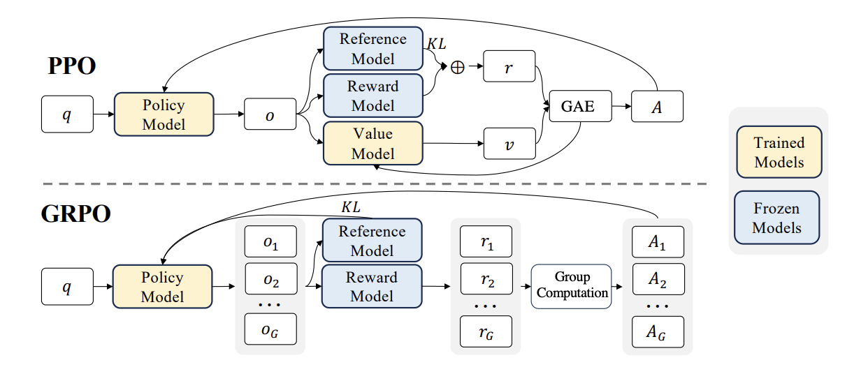
Image: PPO and GRPO; their similarities and differences – source: (Shao et al, 2024). Note that there are variants of PPO that permit generating multiple trajectories, computing their rewards and advantages in one pass (similar to the GRPO figure) but still needing a value model.

It is these – the KL regularisation term and the \(\mu\)-updates – that presents some challenges to overcome (as well as opportunities to leverage as in diffuGRPO) for the use of PPO/GRPO on DLMs, and we will discuss these next… (Note: The rest of this post will go into the weeds on these points and will be more technical.)

♻️ 2. Can we reuse the PPO/GRPO methods that worked for AR-LLMs?

The short answer is… broadly, yes but with the need for some non-trivial modifications to address the issue of how to obtain the likelihood for trajectories from a Masked-DLM. These likelihoods are needed in two places in the PPO/GRPO objective: (i) for an importance sampling weight, as well as (ii) an estimate for the KL-regularisation term.We use the GRPO objective to illustrate (with clipping omitted to reduce clutter in the equation): \(\begin{aligned} L_{GRPO}(\theta) = - \frac{1}{\sum_{i=1}^{G} |o_i|} \sum_{i=1}^{G} \sum_{t=1}^{|o_i|} \\ \bigg[ {\color{red}\frac{\pi_\theta(o_{i,t}|x, o_{i,<t})}{{\left[ \pi_\theta(o_{i,t}|x, o_{i,<t}) \right]}_{\text{no grad}}}} \hat{A}_{i,t} {\color{blue} - \beta D_{\text{KL}}[\pi_\theta \| \pi_{\text{ref}}} ] \bigg] \end{aligned}\)
where \(\pi_{\theta}\) is the current policy and \(\pi_{ref}\) is either the initial (typically obtained via SFT) or some earlier-update \(\pi_{\theta}\).
As we can see:
▪️ the per-token likelihoods (obtained twice, once with gradients through the policy \(\pi_{\theta}\) and another without gradients) are used in the first term (in red). The ratio of these corresponds to an importance sampling on the advantages \(\hat{A}_{i,t}\) (to address that trajectories are coming slightly off-policy in the μ-updates steps);
▪️ the KL-regularisation term is in blue; and this is where the sequence-level likelihoods are used. In practice, this KL estimate is implemented via this form: KL \(= e^r - r - 1\) where \(r = log( \pi_{\theta}(o_{i,t}|x, o_{i,<t}) / \pi_{ref}(o_{i,t}|x, o_{i,<t}) )\). The per-token likelihood for \(\pi_{\theta}\) above can be reused, and only the ones from \(\pi_{ref}\) need to be computed here. For a concrete feel: see the implementation in TRL.

Sidenote: Recent studies (Zhang et al, 2025) and (Tang et al, 2025) have established that there are non-trivial differences relating to a set of fine-grained choices of the method and implementation for the KL divergence estimate. Note that these have implications for online RL of DLMs due to the need to estimate these estimates there (see below). To my mind, these two pieces are recommended reading for RL on DLMs.

Sidenote: If the beta (β) coefficient, which controls the amount of KL-regularisation in PPO/GRPO, is set to be zero, then there is no need for the sequence-level likelihoods. Empirically, there have been reports recently that the KL-regularisation may not be necessary for AR-LLMs (quite likely under certain training setups i.e. hyperparameter setting, modeling choice where the encountered KL divergences between \(\pi_{\theta}\) and \(\pi_{ref}\) are low). See for e.g. (Copet et al, 2025); page 13 of paper.

Computing these likelihood for trajectories is easy for AR-LLMs because of how they factorise sequence probabilities at a token-level; i.e. at each step, the AR-LLM predicts from its vocabulary the most likely token to generate. As a result, it is very easy to compute what an AR-LLM thinks is the likelihood of any sequence of tokens (by chain-rule, i.e. simply summing the log-probabilities for each token of the sequence).See also footnote 27 in the second post of this series.

However, this is not the case 😵‍💫 for Masked-DLMs (and discrete diffusion models generally). Although we do get probabilities for tokens at each step of the diffusion generation process (which is what allows us to decide which token to unmask into), each of these steps is a denoising one that depends on all its preceding steps. In other words, computing sequence probabilities for DLMs require going through multiple denoising steps (from \(T\) to 0). To have to keep doing this for every sampled trajectory during online RL training with PPO/GRPO is very computationally expensive, and will be significantly worse for very long sequences.Although the efficient DLM methods I covered in the previous post (such as Block Diffusion (Arriola et al, 2025)) can help alleviate this, the increase in computation required – compared to what is required in AR-LLMs – will still be substantial. As such, there is a need to establish ways to efficiently, yet as accurately as possible, estimate these likelihoods with the DLM. This is the focus of much research currently and we will look into in the next section.

💡 3. What have been proposed for DLMs?

This section outlines two research trends in online RL algorithms to Masked-DLMs. All of these started with diffuGRPO (Zhao et al, 2025), which landed in Q1 this year and was the first work to explore a way of bringing online RL algorithms to Masked-DLMs. diffuGRPO and the initial wave of research is distinguished by their main contributions for ways to estimate likelihoods with Masked-DLMs, another more recent wave (released in the last month or so) begin to explore extensions for Masked-DLMs with semi-autoregressive generation for longer generations and with more efficiency (e.g. with KV caching).

Efficient likelihood estimation for online RL on Masked-DLMs

Each of the three pieces of work mentioned here proposed a way to do the likelihood estimation. Note that although they were formulated for GRPO, it should be possible to leverage their likelihood approaches for use in a PPO setup.

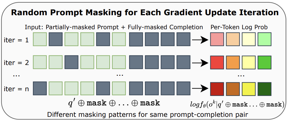
◼️ diffu-GRPO (Zhao et al, 2025): estimate the per-token likelihood of a trajectory by simply doing unmasking in one-step.In practical terms, this is done as follows: for a given prompt \(q_{k}\) append it with a fully-masked continuation (i.e. max sequence generation length) and pass it through the Masked-DLM; this output is the estimated per-token probability distribution (conditioned by the prompt \(q_{k}\)). As noted above, such one-/few-step unmasking does not reflect the multi-step denoising in Masked-DLM – hence and quite importantly, their proposal hinges on (i) the \(\mu\)-updates typically (but not mandatorily) used in GRPO, and (ii) a random masking to the prompt \(q_{k}\) portion of the input (i.e. input = \(q_{k}\) + fully masked continuation). At every of the \(\mu\)-steps, the mask is randomised but always fixed at 15%.See Appendix A of paper: “In gradient update iterations, each token in the prompt is randomly masked with a probability pmask = 0.15 for log-probability estimation.” We can see this as obtaining slightly varied likelihood estimates for a set of inputs closely resembling the prompt \(q_{k}\) which according to the authors “acts a form of regularization for policy optimization”. As for estimating sequence-level likelihood of a trajectory: the authors assume mean-field decomposition (i.e. a series of localized independent distributions can be useful for approximating a complex conditional distribution), allowing them to simply sum the trajectory’s per-token log probabilities to get this estimate. At least two pieces of empirical support are available for diffu-GRPO: (i) (Zhao et al, 2025) reported consistently stronger performance on four different math and puzzle/planning logical problems;See Table 1 and Figure 5 of their paper and (ii) the same approach for obtaining per-token and sequence likelihood was adopted by IGPO (Zhao et al, 2025b) as well and tested successfully on reasoning benchmarks there.

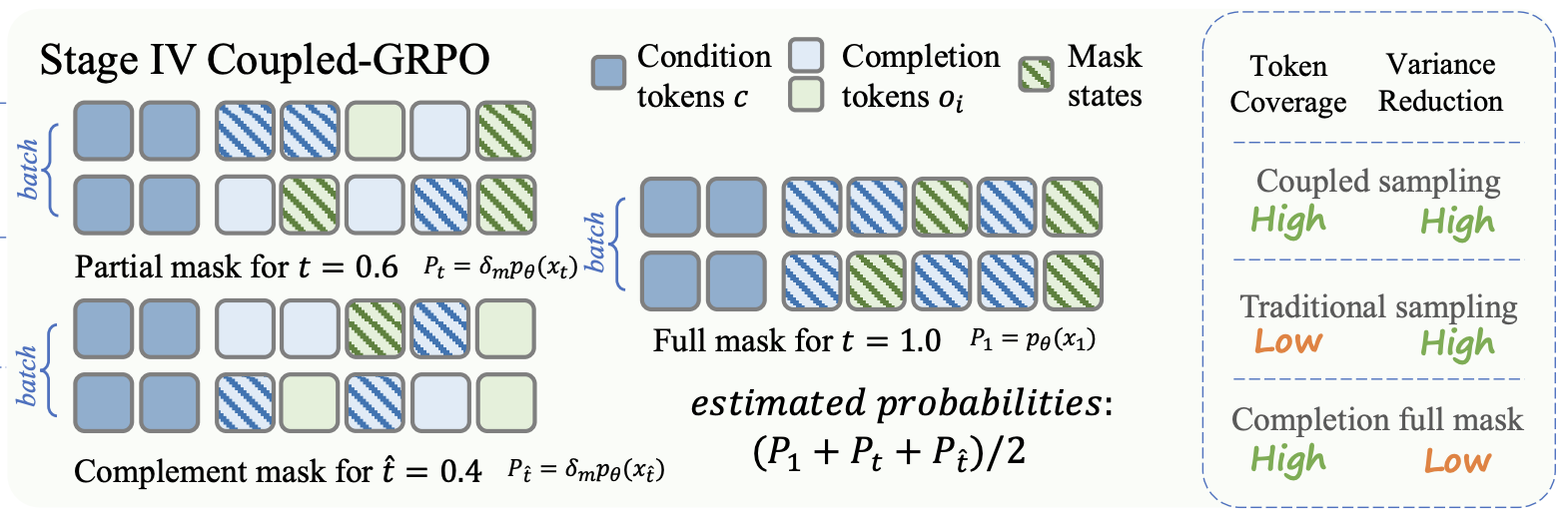
◼️ coupled-GRPO (Gong et al, 2025): departs from diffu-GRPO in that they apply the masking to the continuation portion (i.e. the \(o^k_i\)) for each trajectory. They also use two samples on each trajectory at every \(\mu\)-step for the estimation (compared to diffu-GRPO’s use of only one sample of each prompt \(q_{k}\) at every \(\mu\)-step, which requires much less computation). Each of the two samples masks different, but paired (henced the “coupled” in the name) parts of the continuation.This involves sampling a random timestep \(t\), and then setting the other \(\hat{t}\) so that (i) \(t + \hat{t} = T\), the terminal timestep (i.e. 1.0). Then, what is masked for \(t\) is not masked in \(\hat{t}\) and vice-versa. This ensures that (i) every token in a trajectory is involved once in the estimation giving “each token a non-zero learning signal”, and (ii) it also more closely mimics the denoising generation process in Masked-DLMs (where probabilities are produced on partially masked continuations). coupled-GRPO was used by (Gong et al, 2025) in their training for DiffuCoder, a code generation-focused Masked-DLM, who stated that coupled-GRPO was formulated in response to their findings that diffu-GRPO’s likelihood approximation methods do not “yield a stable reward improvement…, probably because code tasks demand higher token-level generation accuracy than math tasks”. They go on to show that coupled-GRPO leads to stronger performance through stabler rewards (see left and centre chart of Figure 7 in their paper) over diffu-GRPO for coding tasks, as well as for another baseline where they remove the masking coupling of (\(t, \hat{t}\)). Interestingly they also found that coupled-GRPO required sampling trajectories at a higher temperature for success (see right chart of Figure 7 in their paper) which has congruence with similar findings on online RL for AR-LLMs recently (Liu et al, 2025).

◼️ uni-GRPO (Yang et al, 2025): was applied in the training procedure for MMaDA, a Masked-DLM with multi-modal (vision and text) capabilities. It is similar to coupled-GRPO in that it also masks on the continuation to obtain the likelihood estimates. Specifically, the noise for each \(\mu\)-step update is randomly sampled from a uniform distribution (instead of the fixed 15% of the prompt in diffu-GRPO, which also meant that the same timestep (i.e. \(T\)) across all samples was used there). Only one sample on each trajectory at every \(\mu\)-step is taken (i.e. more computation than diffu-GRPO but less than coupled-GRPO). In a departure from the other two approaches, the per-token likelihood is computed with the masked tokens (i.e. this relates to the ELBO of the Masked-DLM),See Equation 3 of the MMaDA paper for uni-GRPO; and compare with Equation 4 of the DiffuCoder paper for coupled-GRPO. and the sequence level likelihood “is then approximated by averaging over masked tokens” (see Equation 4 in paper). Taking the ELBO as the estimate is quite a meaningful departure from the diffu-GRPO and coupled-GRPO approaches, and although it has a theoretical connection to the Masked-DLM training objective, it is not clear that it provides a better estimate for online RL training compared to the case where all tokens are considered (as in coupled-GRPO); nonetheless, it is clear that uni-GRPO outperforms diffu-GRPO (likely due to the larger-sized sampling, i.e. every trajectory every \(\mu\)-step).See comparisons of their performance in Figure 3 in §5.2 of the MMaDA paper and Table 1 of the IGPO paper that also leverages diffu-GRPO.

Other proposals for Masked-DLMs

◼️ wd1 (Tang et al, 2025): proposes a few modifications to the GRPO objective which allow it to be used on a Masked-DLM with likelihood evaluation through one policy only (the current policy \(\pi_{\theta}\)). This is desirable as it is much more computationally efficient compared to the approaches above, which needed to do so for the policy before the \(\mu\)-update (\(\pi_{old}\)) and the reference policy (\(\pi_{ref}\)). Briefly, their approach hinges on shifting from (i) applying the importance sampling to the advantage (as per original PPO; see above) to (ii) applying a reverse KL-divergence penalty.See §3.1 and Equation 3 of their paper. This enables their derivation of an expression on the GRPO objective that only needs likelihood estimates from \(\pi_{\theta}\).In order to obtain their expression of the GRPO objective, it also involves shifting the trajectory sampling (from \(\pi_{old}\)) to a geometric mixture of \(\pi_{old}\) and \(\pi_{ref}\) (see §3.1 of their paper). They report obtaining up to 16% better performance over diffuGRPO on math and logic/puzzle planning benchmarks even without having to do an SFT phase (which is, on the other hand, needed for diffuGRPO to reach reasonable performance).Sidenote: Although, a case could be made that the settings (Tang et al, 2025) use for comparison with diffuGRPO might not be fully like-for-like. Their wd1 objective is obtained assuming the \(\beta\)-controlled KL-regularisation term (see above) is included in the GRPO objective (see their Equation 5). While the final expression of the wd1 objective does away with the KL-regularisation term and does not include it explicitly, the controlling \(\beta\) term remains embedded throughout the wd1 objective (their Equations 9 and 6). Yet in practice \(\beta\) is set to 0 (see “Implementation” in §4 of their paper) for the model trained with wd1 in their experiments, in effect this leaves out the consideration of any KL-regularisation. On the other hand, the \(\beta\) from the original diffuGRPO paper (0.04) was kept (see Table 5 of Appendix B.4). Perhaps it will be helpful to also understand how diffuGRPO performs without the KL-regularisation applied. Notably however, it does not appear that this approach leads to stronger empirical outcomes when compared with uniGRPO.Compare the reported scores on GSM8K and MATH500 by (Zhao et al, 2025b) (refer to Table 1) and (Tang et al, 2025) (refer to Table 3; look at the 256-length results as the other paper used a 256 length setting – see Appendix A there).

◼️ IGPO (Zhao et al, 2025b): shares the same first author as diffu-GRPO, and as mentioned above, uses the same likelihood estimation approach as diffu-GRPO. The novelty here is a procedure to leverage the inpainting capabilities inherent in DLMs (see my first post) to optimise the training efficiency and efficacy of GRPO. In GRPO,Refer to the image of PPO vs GRPO in the margins above for a sense. when the entire group of sampled trajectories for a given prompt \(q_{k}\) (for e.g. a math problem) is zero, this results in no useful signal for the model to update its parameters. IGPO’s proposal assumes access to ground-truth or sufficiently high quality reasoning traces for \(q_{k}\) and to use some segment of the reasoning traces when such zero-reward groups are encountered. Specifically, by “seeding” a fragment of the reasoning trace amongst the masked tokens, we get a chance to steer the Masked-DLM towards generating a trajectory of good quality,It is akin to hinting to Jesse “They have 2 plus 2 apples so that is 4 apples…“ which is then swopped with a zero-reward trajectory from the group. Training with this way to avoid zero-reward update steps led to stabler learning and enabled improvements on math and planning benchmarks over diffuGRPO; but importantly, it also outperforms uniGRPO that requires more samples to be taken for the likelihood estimation (per-trajectory per \(\mu\)-update vs per-prompt per \(\mu\)-update).See Table 1 of their paper (Zhao et al, 2025b).

◼️ TraceRL (Wang et al, 2025): encapsulates some of the latest developments on a few fronts in Masked-DLM research. To summarise, they propose the use of a value model (another DLM) to manage the variance across updates (à la PPO). In addition, they leverage the semi-autoregressive approach of Fast-dLLM (Wu et al, 2025), which I discussed in my previous post, that denoises blocks of tokens auto-regressively with efficiency via the use of approximated KV caches. This has the effect of giving a speed up to trajectory sampling, easing a major bottleneck especially for problems that are best solved with lengthy reasoning traces. To put these extensions together required special treatment (e.g. their §4.3), and this work is notable for putting forward a proposed solution for doing so. They report impressive performance on math benchmarks (87.4 for GSM8K and 94.2 for MATH500) that outperform the other methods listed above in this section,See Table 2 of their paper (Wang et al, 2025); and compare against results report in the other papers. as well as ones for coding. Helpfully, the authors released the TraDo series of 4B/8B parameters Masked-DLMs that they trained with this approach, alongside their codebase.

🤔 4. What’s next?

To sum up, in this post, I started with a general overview of online RL post-training for LLMs. With some common ground established on that, I highlighted the main challenge for extending existing methods for AR-LLMs to Masked-DLMs, which is the issue of how to efficiently and accurately estimate token and sequence likelihoods needed for the PPO/GRPO objective. Finally, I gave an outline for recent work bringing PPO/GRPO to Masked-DLMs, focusing on how they proposed to address this estimation challenge.

This wraps up the first round on the topics I intended to cover in this series; the next posts – probably slightly further out – would look at all the areas I have discussed so far, but with multi-modality in consideration.